


This paper assesses the potential of in situ monitoring to provide a localized index of hydrological drought in Somaliland. It finds that calibrating a lumped groundwater model with a short time series of groundwater level observations substantially improves the quantification of local water availability when compared to satellite-based indices.
By W. A. Veness, A. P. Butler, B. F. Ochoa-Tocachi, S. Moulds, and W. Buytaert
Water Resources Research | Volume 58, Issue 8, August 2022
First published: 08 August 2022
Abstract
Drought early warning systems (DEWSs) aim to spatially monitor and forecast risk of water shortage to inform early, risk-mitigating interventions. However, due to the scarcity of in situ monitoring in groundwater-dependent arid zones, spatial drought exposure is inferred using maps of satellite-based indicators such as rainfall anomalies, soil moisture, and vegetation indices. On the local scale, these coarse-resolution proxy indicators provide a poor inference of groundwater availability. The improving affordability and technical capability of modern sensors significantly increases the feasibility of taking direct groundwater level measurements in data-scarce, arid regions on a larger scale. Here, we assess the potential of in situ monitoring to provide a localized index of hydrological drought in Somaliland. We find that calibrating a lumped groundwater model with a short time series of groundwater level observations substantially improves the quantification of local water availability when compared to satellite-based indices. By varying the calibration length, we find that a 5-week period capturing both wet and dry season conditions provides most of the calibration capacity. This suggests that short monitoring campaigns are suitable for improving estimations of local water availabilities during drought. Short calibration periods have practical advantages, as the relocation of sensors enables rapid characterization of a large number of wells. These well simulations can supplement continuous in situ monitoring of strategic point sources to setup large-scale monitoring systems with contextualized and localized information on water availability. This information can be used as early warning evidence for the financing and targeting of early actions to mitigate impacts of hydrological drought.
Key Points
- Advancements in sensing technologies give renewed feasibility to in situ groundwater monitoring in data-scarce, drought-prone countries
- Calibrating groundwater models with short observation records (weeks) substantially improves on satellite-based drought exposure indicators
- Improved water availability assessment with in situ sensors provides opportunities for better drought early warning and early action
1 Introduction
Drought-prone regions host many of the world’s least developed countries, which are experiencing increasing drought risk as a result of population pressures and increasing drought frequencies (UNDRR, 2015). This is evident in Somalia, where estimated fatalities from the 2011 drought exceeded 250,000 and a further drought in 2017 required humanitarian assistance for 6 million people (FAO, 2018, 2019). Drought early warning systems (DEWSs) aim to monitor and forecast drought risk, enabling early interventions that mitigate the most severe socioeconomic impacts. To formulate this risk, DEWSs require evidence of drought intensity and community exposure collected by monitoring systems (Brown, 2014; UNDRR, 2015).

1.1 Current Drought Monitoring Methods for Early Warning
A range of regional-scale, satellite-based indicators are used to monitor physical drought development. The Standardized Precipitation Index (SPI) is a popular indicator for monitoring meteorological drought (McKee et al., 1993; Van Loon, 2015). The SPI indicates rainfall anomaly compared to the long-term average for that chosen time period (Sheffield et al., 2014). For agricultural drought (Van Loon, 2015), satellite-based indicators are used such as soil moisture and the Normalized Difference Vegetation Index (NDVI; Liang et al., 1994; NASA Worldview, 2022; Tarpley et al., 1984). These indicate available soil moisture for vegetation growth, which in turn indicates crop failure in areas where agriculture is nonirrigated (Brown, 2014; FEWS NET, 2021; FSNAU, 2021; Sheffield et al., 2014). However, in most arid zones during late dry seasons, water availability for human consumption depends on groundwater supply. As such, these surface indicators are not ideal for assessing hydrological droughts—the most intense form of drought that causes water shortages (Kumar et al., 2016; MacAllister et al., 2020; Tallaksen & Van Lanen, 2004; Van Loon, 2015). Nevertheless, these same satellite-based indicators of meteorological and agricultural drought are used by DEWSs to infer the spatial intensity of hydrological drought by proxy because of a paucity of direct groundwater observations (Brown, 2014; FEWS NET, 2021; FSNAU, 2021; Kumar et al., 2016; Sheffield et al., 2014; UCSB, 2021).
In practice, these indicators show abnormally large declines during the early stages of drought (Kchouk et al., 2021), and thus provide some evidence to trigger a national or regional early warning at a good lead-time ahead of the highest intensity phase of drought. However, despite useful lead-times, the spatial accuracy of these indicators is low due to the coarse resolution and measurement uncertainty of the satellite data used as inputs (FSNAU, 2021; Karnieli et al., 2010; Sheffield et al., 2014). Furthermore, the extent to which seasonal changes in these indicators reflect actual underlying groundwater levels is unknown—aquifer recharge and well recovery depends heavily on drainage basin characteristics and human activity. As a result, these coarse physical drought indicators are used by practitioners with caution when determining which communities are most locally exposed to hydrological drought and therefore at risk of water shortages (Karnieli et al., 2010; Kchouk et al., 2021; MacAllister et al., 2020; Okpara et al., 2017).
During drought development, these physical indicators are viewed alongside seasonal climate forecasts from international organizations such as the GHACOF (Greater Horn of Africa Climate Outlook Forum), the Famine Early Warning Systems Network (FEWS NET), the National Oceanic and Atmospheric Administration (NOAA), and the UK Met Office, which give a low-certainty prediction of how the drought may evolve in future months (Brown, 2014; Dinku et al., 2018; FAO, 2021; FEWS NET, 2021; Mwangi et al., 2014). For shorter-range forecasts, the popular United States Geological Survey’s Early Warning Explorer (USGS EWX) tool provides open access to the latest 15-day pentadal rainfall forecasts (UCSB, 2021). Meteorological forecasts are also compromised by a low spatial resolution and high uncertainty, particularly at longer lead-times. Furthermore, the scarcity of national hydrological monitoring programs in Sub-Saharan Africa prevents national agencies from augmenting these forecasts with local data (Brown, 2014; Stephens et al., 2015). Therefore, combining low-resolution indicators of physical drought intensity with these forecasts results in high uncertainty about current and future drought exposure at the local scale (Boluwade, 2020; Dinku et al., 2018; Kumar et al., 2016; Pappenberger et al., 2005).
As a result of these limitations, drought managers, including national agencies and international NGOs, depend on national socioeconomic data to spatially monitor drought exposure through evidence of drought impacts (FAO, 2018; FSNAU, 2021). These data are the primary source of information used to plan and finance early interventions with prioritized communities (Brown, 2014; Buchanan-Smith & McCelvey, 2018; FSNAU, 2021; Stephens et al., 2015). In Somalia and Somaliland, this information is made available in real-time by the United Nations Food and Agriculture Organization’s Food Security and Nutrition Analysis Unit’s (UN FAO FSNAU) Early Warning Early Action dashboard (FSNAU, 2021). It presents monthly data on market prices, livestock prices, migration data, disease prevalence, wages, and nutrition. For example, by October 2016, when the socioeconomic impacts of the 2016/17 drought first became apparent, the socioeconomic indicators had reached the “alarm” phase over 200 times across all of Somalia’s administrative regions, over double the previous year’s level (FSNAU, 2021).
Socioeconomic data are fundamental for monitoring vulnerabilities to drought (Brown, 2014; UNDRR, 2015); however, an over-dependence on socio-economic data for monitoring real-time drought exposure is problematic for DEWSs. Requiring signals from socioeconomic drought impacts for an early warning to be triggered means that opportunities for early, water shortage-mitigating interventions have already been missed. A further limitation is the coarse spatial and temporal resolution of the socioeconomic indicators, with monthly data aggregated by FAO FSNAU in Somalia for each administrative region (Brown, 2014; FSNAU, 2021). This has the effect of smoothing out localized drought impacts, to the extent that DEWSs have little information on relative exposure at the community level. This can lead to poorly targeted and ill-timed interventions which fail to mitigate water shortages and the cascading secondary impacts of malnutrition, economic losses, community displacement, famine, and conflict in the most exposed regions (Brown, 2014; FAO, 2014; MacAllister et al., 2020; Stephens et al., 2015).
1.2 Modern Sensors for In Situ Groundwater Monitoring
The limitations of using regional methods to monitor hydrological drought exposure illustrate the need for alternatives. Despite advice in 2003 by UN FAO that data on groundwater level fluctuations are “essential as a basis for management” (FAO, 2003), methods to monitor drought still widely omit in situ groundwater data (Lewis & Liljedahl, 2010). Reasons have included the high economic cost of data collection, the labor-intensive nature of monitoring, difficulties with community participation, and a lack of hydrological expertise to process the data (Ajoge, 2019; Calderwood et al., 2020; Frommen et al., 2019).
Advances in sensing technology have reduced the cost and complexity of in situ monitoring to a level where it can now be implemented on an unprecedented scale (Buytaert et al., 2016; Calderwood et al., 2020; Paul & Buytaert, 2018). Modern automatic sensors have lower costs, greater accuracy, higher-frequency measurements, real-time telemetry, longer battery lives, and now require less labor and expertise for installation and data processing (Calderwood et al., 2020; Paul & Buytaert, 2018). However, the long-term maintenance of in situ sensors remains resource intensive. Therefore, in proposing a scalable method for groundwater monitoring, understanding the optimal duration of in situ data collection for useful and cost-effective monitoring is crucial.
Here, we explore whether short-term, high-frequency monitoring can be used to calibrate a groundwater model sufficiently to enable accurate simulations of groundwater availability at the local scale, using a case study of three abstraction wells in Maroodi Jeex, in the self-declared independent republic of Somaliland. The paper is structured as follows. First, we describe the groundwater model and calibration procedure. Then, by varying the calibration length between 1 and 30 weeks, we assess the value of additional calibration weeks for model performance. From this, a 7-week calibration is used to evaluate how effectively the model simulates observed groundwater availability compared to satellite-based proxy indicators. The calibrated wells are then simulated between 2015 and 2020, to illustrate how the model can be used to index hydrological drought during the 2016/17 and 2019 Horn of Africa drought events. This is followed by a discussion of how this method can be scaled-up to a large number of wells, and how the information can be used to inform the planning of early and effective interventions during droughts.
2 Method
2.1 Modeling Approach
In data-scarce regions, simple conceptual groundwater models are favored over process-driven models (Beven, 2001; Mackay et al., 2014). Here, we use a modified version of the quasi-physically based AquiMod model to simulate the local water table in response to satellite-derived rainfall and evapotranspiration rates (Mackay et al., 2014). The model (fully described in Supporting Information S1) provides a simple and efficient method to simulate time-dependent well water levels based on a conceptual representation of groundwater systems, with a parameter set small enough to deploy automated calibration procedures at low runtimes (Beven, 2001; Mackay et al., 2014). Model inputs, comprised of daily rainfall and actual evapotranspiration values for an area surrounding the pumping well, were obtained from satellite data (Maidment et al., 2017; Sheffield et al., 2014). The model was calibrated against in situ groundwater level data using a Monte Carlo approach (Mackay et al., 2014; Pianosi et al., 2015).
2.2 Input Data
Daily precipitation and actual evapotranspiration data for the period 2015–2020 were obtained from, respectively, TAMSAT (Tropical Applications of Meteorology using Satellite Data; Maidment et al., 2017) and AFDM (African Flood and Drought Monitor; Sheffield et al., 2014). For point-scale applications, there is higher uncertainty associated with the daily rainfall product when used at its finest 4-km spatial resolution, particularly when employing temporal downscaling from the initial 5-day cumulation product. To reduce this uncertainty, we averaged daily rainfall over a 40-km square (Maidment et al., 2017). Daily AFDM actual evapotranspiration data have a spatial resolution of 27 km. The lower spatial variability of evapotranspiration means it is associated with less uncertainty than the rainfall input (Sheffield et al., 2014). Average evapotranspiration over 54 × 54 km was calculated for model input.
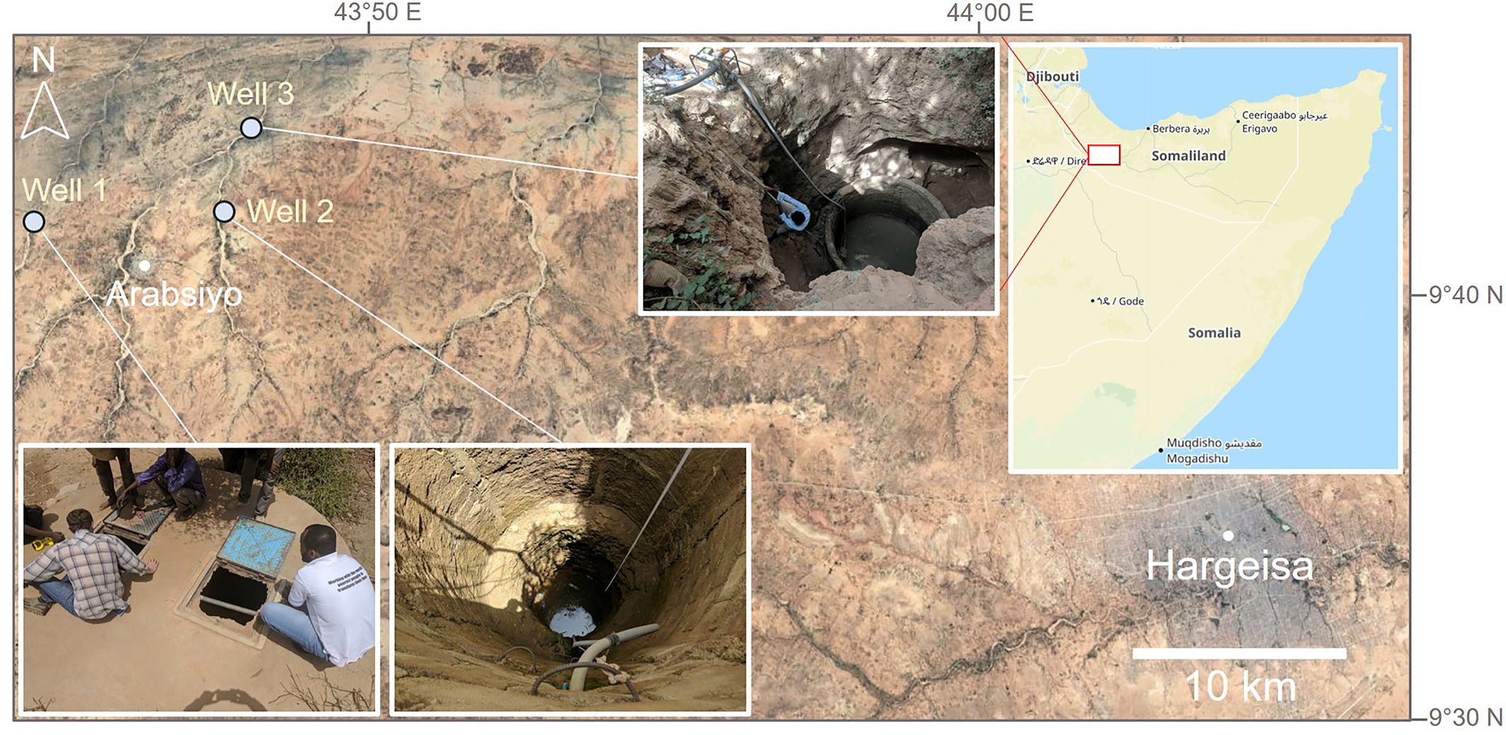
Groundwater levels at 15-min intervals were obtained using pressure transducers in three shallow, large-diameter wells in Maroodi Jeex, Somaliland. Shallow wells provide an ideal target for DEWSs because they typically run dry before deeper boreholes and thus display an earlier drought signal in rural areas (MacAllister et al., 2020). Sensor installation took place on 21 July 2017, at sites <10 km apart (Figure 1).

Figure 1
Location of the three shallow, large-diameter wells in Maroodi Jeex, Somaliland.
The selected wells, although geographically close, displayed markedly different behavior due to differences in local geology, construction, and usage (Figures 4b–4d). Although they sit within a common unit—a weathered, unconfined section of the Upper Cretaceous Yesomma (Nubian) Sandstone—local differences in porosity, conductivity, and specific yield were observed due to regional interfingering of clastic and carbonate facies (Ali, 2009, FAO SWALIM, 2021). This heterogeneous aquifer was therefore a suitable location to test the modeling approach under varying unconfined aquifer properties.
A 7-month time series of data was collected for the three wells, which reflected some of the outstanding challenges of continuous data collection in this environment including logistics, battery supply, and staffing (Paul & Buytaert, 2018). The three data sets were each used for separate calibrations of the modified AquiMod model.
2.3 Groundwater Model
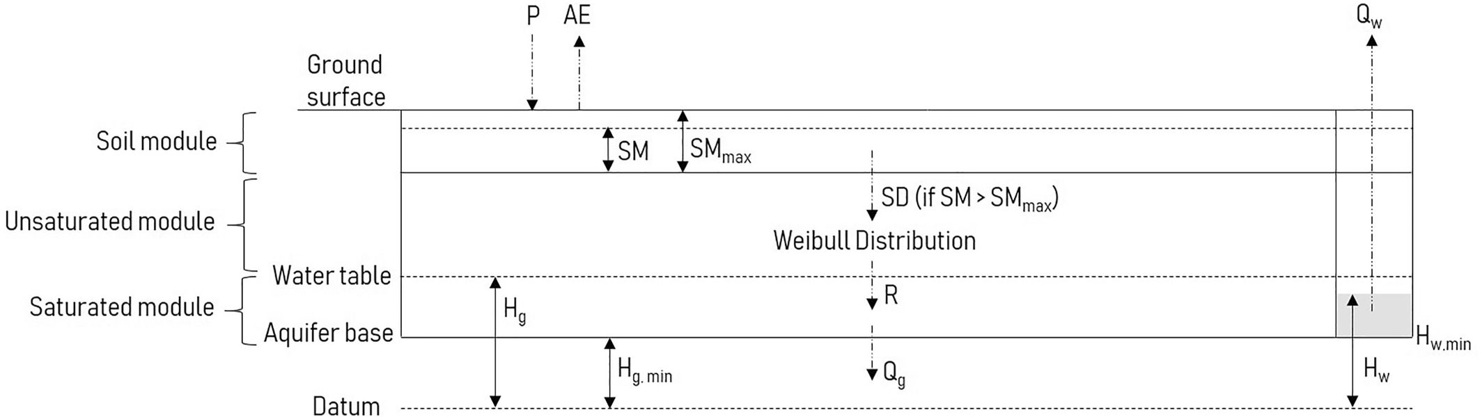
We use a modified form of AquiMod (Mackay et al., 2014) to estimate aquifer recharge (R) and calculate groundwater drainage (Qg), outputting a daily water balance for the well. The unconfined (saturated) aquifer module is represented as a single locally homogeneous and isotropic layer, above which is an equally homogeneous unsaturated module that is, in turn, overlain by a soil module (Figure 2). Precipitation (P) enters the top soil module following losses due to actual evapotranspiration (AE). If the soil moisture (SM) exceeds the maximum soil moisture capacity (SMmax), the surplus water becomes soil drainage (SD) to the unsaturated zone module. This drainage is then delayed by being distributed over time using a Weibull distribution to provide recharge (R) to the saturated module. In the saturated container, recharge from soil drainage is the sole input.

Figure 2
Modified AquiMod lumped catchment regional model for a single unconfined aquifer layer.
The main output is the volume of groundwater drained (Qg), which represents losses from the local groundwater system through regional processes. This assumes that the groundwater level drains from the system at a rate proportional to its height (Hg) above the minimum drainage level (Hg,min; Cuthbert, 2014). In this study, Qg is adapted from the single-layer AquiMod model in Mackay et al. (2014), by lumping the parameters used to calculate its value. This allows the model to be reduced to a single vertical spatial dimension (Figure 2), where Qg is calculated according to the difference in the height of the groundwater level (Hg) above the base of the aquifer (Hg,min, which is set equal to the pump inlet depth, Hw,min, as this is the “effective” locally accessible depth of aquifer) factored by a time constant “τ” [day−1]. Therefore, “τ” is an empirical, lumped parameter open for calibration, representing the combined effects of groundwater flow from well to outlet, aquifer leakage, and nearby abstractions that can all combine to decrease the local water level (Mackay et al., 2014). This simplification removes the need to represent groundwater flow using Darcy’s law and thus avoids needing to define hydraulic conductivity and distances to outlets on the boundary of the model. It improves the feasibility of a short calibration period by removing two additional parameters from the procedure, which in turn increases the sensitivity of τ to improve the calibration (Beven, 1989). The model conceptualization and the adapted equations are fully described in Supporting Information S1.
Equation 1 calculates the change in groundwater level (Hg) for each time step, by dividing the balance between the total recharge (R), drainage (Qg), and well-abstraction (Qw) by specific yield (Sy) and a nominal area around the well (A)
 (1)
(1)
If the area is sufficiently large whereby |R| and |Qg| >> |Qw|, as is common in shallow wells with low abstraction volumes, then the impacts on the regional groundwater level due to abstraction from the modeled well can be ignored, and the recharge and groundwater drainage can be modeled as fluxes (r and qg, respectively). Equation 1 is then discretized using an explicit forward difference scheme and integrated on a time step of 1 day, using daily recharge values obtained from the soil and unsaturated zone modules. This gives a continuous daily time series of the unpumped groundwater level elevation (Hg) for each well site (Figures 4b–4d; Veness et al., 2022).
2.4 Calibration Method
We calibrated the model using Monte Carlo and Global Sensitivity Analysis (GSA) methods (Ochoa-Tocachi et al., 2018; Pianosi et al., 2015). Following sensitivity analysis, we focused on calibrating four sensitive parameters, while setting the remaining parameters to fixed values estimated from prior understanding of the aquifer and general hydrological systems. We sampled 10,000 combinations from a uniform distribution using Latin Hypercube Sampling (LHS; McKay et al., 1979). Input ranges were set following a manual calibration and an initial scoping study of parameter sensitivity.
In this study, the AquiMod calibration is modified so that Hg,i is calibrated to the maximum water level in the observed data for day “i” (Hw,i,max). In abstraction wells, pumping causes partial recovery (Hw) to the unpumped water table (Hg). This difference is at a minimum following well recovery, immediately before the onset of the following abstraction event. Therefore, calibrating Hg,i to these daily observed peaks in groundwater level changes Hg to a simulation of “available groundwater level” in that well. This requires an assumption that daily partial well recoveries reach a constant distance from the natural unpumped water level, which was considered appropriate based on the observed well recoveries. In data sets where Hg,i − Hw,i ≠ constant, this method can be coupled to a pumping model to include the effect of variable abstraction rates on the modeled water level (see Supporting Information S1). For example, given the variable abstraction drawdowns and partial recoveries seen in Well 3 (Figure 4d), coupling a pumping model may improve the fit in future implementations.
2.5 Calibration Length Analysis
To assess the relationship between calibration length and model performance, the calibration period was varied at weekly intervals between 1 and 30 weeks. The Root Mean Square Error (RMSE) score was calculated for the full 30 week combined calibration and validation period each time (Pianosi et al., 2015). This method highlights an “optimal” calibration period within the 30-week range for groundwater modeling in this context, once additional weeks of in situ observations have diminishing value in improving model performance and the challenges of monitoring outweigh the benefits. Following this, a 7-week calibration was selected as a suitable duration and used for further analysis.
The best scoring parameter sets from the 7-week calibrations at each well (4.5 week for Well 3 due to a shorter data set) were used in a 23-week validation (Table 1). The fit of the validations was compared to satellite-based indicators of NDVI, soil moisture and SPI-3 (Figure 4), as well as uncalibrated simulations of the original AquiMod model at each well that define literature-derived parameter values (see Supporting Information S1; Ascott et al., 2020; Domenico & Schwartz, 1990; FAO SWALIM, 2021; Jackson et al., 2016; Lohman, 1972; Mackay et al., 2014).
Parameter Input Ranges, Calibrated Parameter Values and Root Mean Square Error (RMSE) Scores for the Top Scoring 7-Week Calibration Sets at Wells 1, 2, and 3
| Parameter | Units | Input range (Well 1) | Calibration (Well 1) | Input range (Well 2) | Calibration (Well 2) | Input range (Well 3) | Calibration (Well 3) |
|---|---|---|---|---|---|---|---|
| Sy | – | 0.05–0.12 | 0.0753 | 0.005–0.01 | 0.00720 | 0.025–0.045 | 0.0340 |
| τ | day−1 | 5e−4–1e−3 | 7.29e−4 | 5e−5–1.5e−4 | 1.02e−4 | 2e−4–4e−4 | 2.65e−4 |
| k (Weibull) | – | 3–15 | 3.67 | 3–8 | 5.24 | 3–30 | 19.0 |
| λ (Weibull) | – | 10–30 | 20.1 | 18–30 | 23.9 | 10–30 | 14.1 |
| Hg (t = 0) (fixed) | m | 1.17 | 1.17 | 1.9 | 1.9 | 1.65 | 1.65 |
| SMmax (fixed) | m | 0.005 | 0.005 | 0.005 | 0.005 | 0.005 | 0.005 |
| SMinitial (fixed) | m | 0 | 0 | 0 | 0 | 0 | 0 |
| Hg,min (fixed) | m | 0 | 0 | 0 | 0 | 0 | 0 |
| RMSE (calibration) | m | 0.0577 | 0.339 | 0.0423 | |||
| RMSE (validation) | m | — | 0.0997 | — | 0.982 | — | 0.218 |
Satellite-based indices were downloaded to compare how well they represent these observed groundwater levels by proxy. NDVI and Soil Moisture Active Passive (SMAP) data were downloaded at Well 2’s coordinates from NASA Worldview (NASA Worldview, 2022), and daily SPI-3 values from Princeton’s African Flood and Drought Monitor (5). NDVI is generated by the Aqua Moderate Resolution Imaging Spectroradiometer (MODIS) instrument and downloaded in 16-day intervals at a 250-m spatial resolution (NASA Worldview, 2022). The SMAP layers show a daily composite of surface soil moisture in cm3/cm3, calculated by the Single Channel Algorithm V-Pol for the daily half-orbit passes by the SMAP radiometer and posted to the 9-km EASE-Grid 2.0 (NASA Worldview, 2022). SPI-3 is calculated from bias-corrected Multi-satellite Precipitation Analysis (TMPA) and hybrid reanalysis data (Huffman et al., 2007; Sheffield et al., 2014).
2.6 Model Simulations During 2017 and 2019 Droughts
Using the same calibration parameters (Table 1), the models were simulated from January 2015 to December 2020 using historic rainfall and evapotranspiration as inputs (Maidment et al., 2017; Sheffield et al., 2014). The initial heads to start the model have been estimated by comparing January 2015 SPI-3/6/12 values with January 2018, for which there is corresponding observed groundwater level data, and assessing a likely groundwater level relative to the January 2018 level. The 2016/17 drought event is highlighted from the date the Somalia government declared drought (Guled, 2017) to the final observed rains of the following Gu rainy season. The 2019 drought is highlighted from the declaration date of drought emergency made by Oxfam (Barter, 2019), to the final Gu rains that year.
A critical level is defined for each well, below which the regular abstraction drawdowns observed during the dry season would not be possible. This is due to the water level falling below the pump inlet depth during abstraction drawdown, causing a “dry pump.” A “regular” dry season drawdown was calculated as the mean drawdown depth (m) during the final 50 observed dry-season abstractions at each well. This value was then added to the pump inlet depth (Hw,min) to calculate the well’s critical level.
3 Results and Discussion
3.1 Calibration Length Analysis
The analysis shows that there is little further improvement in calibration performance after extending to 5 weeks (Figure 3). At this period (3 weeks at Well 3), the calibration window is long enough to include the start of the wet season, with groundwater level observations that have increased due to recharge. This causes the recharge parameters of Sy, λ, and k to become sensitive and trained in the calibration. It is therefore essential to have a calibration period that captures observations from both the wet and dry seasons for sufficient calibration of the model. The remaining error in RMSE at the longest calibrations will be sourced from input inaccuracies from the rainfall and evapotranspiration data, as well as modeling uncertainty with processes uncaptured by the simple, lumped parameter model (Ascott et al., 2020; Mackay et al., 2014). Following this analysis, a 7-week calibration period covering equal intervals of dry and wet season conditions is selected as a suitable time window (Figures 4b–4d). The three calibrated wells achieve an efficient fit to the observed water levels in validation, with RMSE scores of 0.0997, 0.982, and 0.218 m respectively.

Figure 3
Root Mean Square Error (RMSE) for the full calibration and validation period, with calibration lengths varied at weekly intervals.

Figure 4
(a) Normalized satellite-based proxy indicators of physical drought intensity compared to Well 2’s observed daily maximum water levels. Calibrations of (b) Well 1, (c) Well 2, and (d) Well 3 are shown to compare performance with the proxy indicators and an uncalibrated AquiMod groundwater model. Observed water levels and the corresponding calibration targets set at the daily maxima are shown for comparison of fit.
3.2 Model Performance
The satellite-based indicators (Figure 4a) are not suitable proxies of local groundwater level. Soil moisture approaches its minimum months before the observed wells and remains at a flat minimum level throughout the long dry season. SPI-3 represents rainfall anomaly instead of absolute rainfall, so is unlikely to follow groundwater levels closely due to its calculation (6). NDVI shows the closest fit to observed groundwater levels, but it underestimates the dry season water level decline and suffers from a low temporal resolution. This potential for NDVI to misrepresent ground conditions was highlighted recently by UN FAO SWALIM, who removed it as a parameter from their Combined Drought Index DEWS platform, citing a “poor correlation” between NDVI and ground information (FAO SWALIM, 2022).
Compared to the regional indicators, the calibrated model provides a substantially improved representation of observed groundwater levels (Figures 4b–4d). The locally calibrated simulations capture the unique response of each well to recharge and dry periods, giving a more reliable indication of water availability. In comparison, the poor performance of the uncalibrated groundwater model highlights the need for a local calibration, as literature-derived parameters fail to capture differences in well and local aquifer properties.
There are remaining limitations in the model performance, with compounding uncertainties from input data, lumped model design, and the short calibration (Mackay et al., 2014). Although it is difficult to quantify the contribution of individual uncertainties to model error, validation tests of this approach when implementing it in a new region will highlight if there are local causes of significant error requiring factoring into the modular AquiMod model (Ascott et al., 2020). It is recommended to extend this validation testing in a sample of wells to multiyear durations, to assess if any interannual variabilities in aquifer or human behaviors affect the performance of parameters fixed by the short calibration. In any application, the outstanding uncertainty of simulations and the potential causes and effects of interannual variability must be carefully conveyed to users (Twomlow et al., 2022).
The required model performance depends on the use case and the specific decisions being informed by the real-time simulations (Maxwell et al., 2021; Twomlow et al., 2022; Zulkafli et al., 2017). This can be modified to an extent, by adjusting the model setup or extending calibration durations where practical. In some implementations, strategic wells within the simulated monitoring network may warrant continuous monitoring to reduce monitoring uncertainties further. However, in drought-prone areas where no groundwater information is currently available and communication between communities and intervening authorities are weak, short monitoring may provide best value and practicality for generating useful evidence to support early interventions by stakeholders who are increasingly adopting “no regrets” approaches to anticipatory action (Lentz et al., 2020).
3.3 Simulating the 2017 and 2019 Droughts
To demonstrate the model’s use as a localized index of groundwater availability, the calibrated wells are simulated during the two most recent droughts in Somaliland (Figure 5). These water levels are put into the context of local water availability by plotting each well’s critical level, below which a full, regular abstraction drawdown would not be possible (Section 2.6).

Figure 5
2015–2020 simulations of the three wells using the 7-week calibration parameters. Water levels are normalized to the distance between the top of the well and the pump inlet depth. The two droughts are indicated from the dates that humanitarian crises were declared by the Somalia president (2017; Guled, 2017) and Oxfam (2019; Barter, 2019). The critical level is the level below which the mean observed dry-season abstraction drawdown would not be possible due to water level falling below the pump inlet.
The lowest water levels are seen during the two documented droughts (Figure 5; Barter, 2019; FEWS NET, 2021; FSNAU, 2021; Guled, 2017). Wells 1 and 2 fall below their critical level during the two droughts, indicating that regular abstraction drawdowns would have been restricted. Well 3 remained above its critical level throughout. This indicates that Wells 1 and 2 suffered abstraction shortages during the two droughts, which may have required interventions depending on the function of the well, the availability of alternative water sources and the socioeconomic context of the community using it for water supply.
During long dry seasons where recharge is typically zero from January to early March (Figure 5; Maidment et al., 2017), this real-time visualization of water level decline enables a visual trajectory of the lead-time before the wells reach their critical levels. Users can also compare real-time water levels to simulations of water levels during previous drought years, such as 2017 (Figure 5), to contextualize the severity of the real-time water shortage with their experiences or understanding of previous droughts in that region (Campbell et al., 2021; Sword-Daniels et al., 2016). For both hydrologists and nonexperts, this direct comparison connects an understanding of the potential impacts of current water shortages, as well as the actions that can be taken to mitigate them based on learned lessons (Hillbruner & Moloney, 2012).
Forecast inputs have not been explored here, as they suffer from high cascading uncertainties at lead-times beyond 1 week (Pappenberger et al., 2005; Walker et al., 2019). However, future development of this approach may explore the use of meteorological forecast data to simulate future water levels. On a lead-time of 1–2 weeks, data sets such as the 15-day CHIRPS-GFES pentadal rainfall forecasts can be used (UCSB, 2021). If forecasting months ahead, seasonal forecasts from GHACOF (56) can be used to project future water levels under different rainfall scenarios. This can further support decision-makers in planning interventions, by translating how water levels will respond to upcoming surface conditions.
4 Conclusions
This study finds that groundwater models with short calibrations, capturing 1–2 months of wet and dry season observations, offer substantial improvements in quantifying local groundwater availability when compared to satellite-based indicators used to infer this by proxy (Brown, 2014; FEWS NET, 2021; FSNAU, 2021; Kumar et al., 2016; UCSB, 2021). Furthermore, by presenting water levels relative to each well’s unique critical depth, the method provides a local and contextualized indicator that translates water levels to water availability (4; Sutanto et al., 2019).
By using modern sensors with short observation periods, the barriers to scaling-up these methods in a national-scale monitoring system are reduced. The low cost of the sensors addresses the economic hurdle of monitoring (Paul et al., 2020), and the short residence time means the sensors can be relocated to calibrate a large number of wells. Short, high-frequency measurements also capture abstraction behaviors, enabling contextualizing calculations of each well’s critical water level. Although serious challenges and ethical considerations in implementation remain, such as monitoring system governance, sensor security, and community consent to participation (Buytaert et al., 2014; Paul & Buytaert, 2018), this study highlights the renewed technical feasibility of large-scale groundwater monitoring for hydrological drought monitoring and early warning.
For DEWSs, maps and hydrographs of real-time water levels can be presented alongside simulated water levels during historic drought events to place the real-time hydrological drought intensity into context (Twomlow et al., 2022). Stakeholders with lived experience of previous droughts can then interpret the likely processes and socioeconomic impacts that will arise from groundwater levels being higher or lower than previous drought years (Campbell et al., 2021; Hillbruner & Moloney, 2012). For national and humanitarian stakeholders, spatial maps of relative drought exposure can inform the national programming of anticipatory action and emergency response. Furthermore, with forecast-based financing systems in need of more evidence to confidently trigger earlier anticipatory financing release (Stephens et al., 2015), maps of drought exposure can be used to trigger the release of intervention financing. A recent growth in parametric insurance for drought, seeking to payout ahead of peak impacts based on hydrological parameter threshold exceedance, also suggests demand for groundwater availability as a localized parameter to index these policies (Okpara et al., 2017). For local stakeholders, access to localized, community-scale information enables actions that mitigate water shortages. Early interventions include site visits, advice and technical assistance, scaling-up proportionately to emergency water supplies, other lifestyle-sustaining supplies, and cash transfers (Brown, 2014; Stephens et al., 2015; Wendt et al., 2021).
The methodology outlined in this report is deliberately parsimonious, and it aims to serve as a demonstration of technical feasibility upon which greater complexity can later be introduced. There are considerable limitations in these methods from a traditional hydrological modeling perspective, from input uncertainties to the lumping of model parameters and the use of empirical “critical level” calculations (Mackay et al., 2014; Maidment et al., 2017; Sheffield et al., 2014). However, groundwater modeling in a data-scarce region is intrinsically bound to modeling limitations that cannot be resolved without collecting extensive field data, and this is not a feasible requirement across a monitoring network in this context (Beven, 2001). Further development of this approach should therefore focus on more validation testing of short calibrations in larger pilot schemes, while resolving the degree of uncertainty that is acceptable for users in guiding specific decisions and actions that mitigate water shortages (Maxwell et al., 2021; Zulkafli et al., 2017). Monitoring systems can then be designed that equilibrate practical feasibility with acceptable uncertainty and simulation accuracy (Maxwell et al., 2021).
Drought-prone, data-scarce regions such as the Horn of Africa are challenging environments for modeling, yet these areas can benefit the most from groundwater models to improve drought monitoring and early warning. Overcoming these challenges requires innovative approaches in both data collection and analysis to generate useful, decision-informing early warning information (Nature Sustainability, 2021). Therefore, this study proposes a viable method of generating a useful, localized groundwater availability index for DEWSs and anticipatory actions, that remains mindful of the fundamental requirement of a groundwater monitoring solution to be technically and practically feasible (Beven, 1989).
Acknowledgments
This research was funded by the UK Natural Environment Research Council [NE/S007415/1] and project partners Concern Worldwide UK, whose contribution was funded by the UK AID (FCDO) and the Building Resilient Communities in Somalia (BRCiS) consortium. The authors would like to thank Paz Lopez-Rey, Kenneth Oyik, John Heelham, Dustin Caniglia, Khaled Esse Haibe, and Haron Emukele for their support with fieldwork. Thanks also to Imperial College London’s Grantham Institute for their support through the doctoral training program.
Open Research
Data Availability Statement
Supporting Information
| Filename | Description |
|---|---|
| 2022WR032165-sup-0001-Supporting Information SI-S01.docx1.2 MB | Supporting Information S1 |
Please note: The publisher is not responsible for the content or functionality of any supporting information supplied by the authors. Any queries (other than missing content) should be directed to the corresponding author for the article.
References
- (2019). Using citizen science in monitoring groundwater levels to improve local groundwater governance, West coast, South Africa (pp. 27). University of Western Cape Magister Scientiae MSc (Environ & Water Science).
- (2009). Geology and coal potential of Somaliland. International Journal of Oil, Gas and Coal Technology, 2(2), 168– 185. https://doi.org/10.1504/ijogct.2009.024885
- , , , , , , et al. (2020). In situ observations and lumped parameter model reconstructions reveal intra-annual to multidecadal variability in groundwater levels in Sub-Saharan Africa. Water Resources Research, 56, e2020WR028056. https://doi.org/10.1029/2020WR028056
- (2019). Poor rains, persisting drought deepens crisis in Somalia and Somaliland. Oxfam in Horn, East and Central Africa. Retrieved from https://heca.oxfam.org/latest/press-release/poor-rains-persisting-drought-deepens-crisis-somalia-and-somaliland
- (1989). Changing ideas in hydrology—The case of physically-based models. Journal of Hydrology, 105(1–2), 157– 172. https://doi.org/10.1016/0022-1694(89)90101-7
- (2001). How far can we go in distributed hydrological modelling? Hydrology and Earth System Sciences, 5(1), 1– 12. https://doi.org/10.5194/hess-5-1-2001
- (2020). Remote sensed-based rainfall estimations over the East and West Africa regions for disaster risk management. ISPRS Journal of Photogrammetry and Remote Sensing, 167, 305– 320. https://doi.org/10.1016/j.isprsjprs.2020.07.015
- (2014). Science for Humanitarian Emergencies and Resilience (SHEAR) scoping study: Annex 3—Early warning system and risk assessment case studies. SHEAR Technical Report.
- , & (2018). A review of community-centered early warning early action systems. Concern Worldwide Technical Report. Retrieved from https://admin.concern.net/sites/default/files/media/migrated/community_centered_early_warning_early_actions.pdf
- , , , , & (2016). Citizen science for water resources management: Toward polycentric monitoring and governance? Journal of Water Resources Planning and Management, 142, 01816002. https://doi.org/10.1061/(asce)wr.1943-5452.0000641
- , , , , , , et al. (2014). Citizen science in hydrology and water resources: Opportunities for knowledge generation, ecosystem service management, and sustainable development. Frontiers in Earth Science, 2, 26. https://doi.org/10.3389/feart.2014.00026
- , , , & (2020). Low-cost, open source wireless sensor network for real-time, scalable groundwater monitoring. Water, 12(4), 1066. https://doi.org/10.3390/w12041066
- , , , , & (2021). Living with water: Documenting lived experience and social-emotional impacts of chronic flooding for local adaptation planning. Cities and the Environment, 14(1), 4.
- (2014). Straight thinking about groundwater recession. Water Resources Research, 50, 2407– 2424. https://doi.org/10.1002/2013WR014060
- , , , , , , & (2018). Validation of the CHIRPS satellite rainfall estimates over eastern Africa. Quarterly Journal of the Royal Meteorological Society, 144(1), 292– 312. https://doi.org/10.1002/qj.3244
- , & (1990). Physical and chemical hydrogeology. New York: John Wiley & Sons.
- FAO. (2003). Re-thinking the approach to groundwater and food security. FAO Water Reports No. 24. Rome.
- FAO. (2014). Community-based early warning systems: Key practices for DRR Implementers. A field Guide for disaster risk Reduction in Southern Africa: Key Practices for DRR Implementers. Retrieved from http://www.fao.org/3/a-i3774e.pdf
- FAO. (2018). Horn of Africa—Impact of early warning early action. Protecting pastoralist livelihoods ahead of drought. FAO Report. Rome.
- FAO. (2019). Proactive Approaches to Drought Preparedness—Where are we now and where do we go from here? FAO White Paper. Rome.
- FAO. (2021). GIEWS—Global Information and Early Warning System. Food and Agriculture Organization of the United Nations. Retrieved from http://www.fao.org/giews/en/
- FAO SWALIM. (2021). FAO SWALIM: Somalia water and Land information management drought monitoring. FAO SWALIM: Somalia Water and Land Information Management. Retrieved from http://www.faoswalim.org/water-resources/drought/drought-monitoring
- FAO SWALIM. (2022). FAO SWALIM: Somalia water and land information management combined drought index. FAO SWALIM: Somalia Water and Land Information Management. Retrieved from https://cdi.faoswalim.org/index/cdi
- FEWS NET. (2021). Famine early warning systems network. Retrieved from https://fews.net/
- , , & (2019). Participatory groundwater monitoring in India—Insights from a case-study in Jaipur. Geophysical Research Abstracts, 21, EGU2019-1543.
- FSNAU. (2021). The FSNAU early warning early action dashboard. FSNAU. Retrieved from https://fsnau.org/special-content/fsnau-early-warning-early-action-dashboard
- (2017). Somalia’s new leader declares drought national disaster. Associate Press. Retrieved from https://apnews.com/article/97d80c7f1d0b494f9c55578a2134fa88
- , & (2012). When early warning is not enough—Lessons learned from the 2011 Somalia Famines. Global Food Security, 1(1), 20– 28. https://doi.org/10.1016/j.gfs.2012.08.001
- , , , , , , et al. (2007). The TRMM Multisatellite Precipitation Analysis (TMPA): Quasi-global, multiyear, combined-sensor precipitation estimates at fine scales. Journal of Hydrometeorology, 8(1), 38– 55. https://doi.org/10.1175/jhm560.1
- , , , , & (2016). Reconstruction of multi-decadal groundwater level time-series using a lumped conceptual model. Hydrological Processes, 30(18), 3107– 3125. https://doi.org/10.1002/hyp.10850
- , , , , , , et al. (2010). Use of NDVI and land surface temperature for drought assessment: Merits and limitations. Journal of Climate, 23(3), 618– 633. https://doi.org/10.1175/2009jcli2900.1
- , , , & (2021). A geography of drought indices: Mismatch between indicators of drought and its impacts on water and food securities. Natural Hazards and Earth System Sciences, 22, 323– 344.
- , , , , , , et al. (2016). Multiscale evaluation of the Standardized Precipitation Index as a groundwater drought indicator. Hydrology and Earth System Sciences, 20(3), 1117– 1131.
- , , , & (2020). Hindsight? The ecosystem of humanitarian diagnostics and its application to anticipatory action. Boston: Feinstein International Center, Tufts University.
- , & (2010). Groundwater surveys in developing regions. Air, Soil and Water Research, 3. https://doi.org/10.4137/aswr.s6053
- , , , & (1994). A simple hydrologically based model of land surface water and energy fluxes for general circulation models. Journal of Geophysical Research, 99(D7), 14415– 14428. https://doi.org/10.1029/94JD00483
- (1972). Ground-water hydraulics. Geological Survey Professional Paper 708.
- , , , , & (2020). Comparative performance of rural water supplies during drought. Nature Communications, 11(1), 1099. https://doi.org/10.1038/s41467-020-14839-3
- , , & (2014). A lumped conceptual model to simulate groundwater level time-series. Environmental Modelling & Software, 61, 229– 245. https://doi.org/10.1016/j.envsoft.2014.06.003
- , , , , , , et al. (2017). A new, long-term daily satellite-based rainfall dataset for operational monitoring in Africa. Scientific Data, 4, 170063. https://doi.org/10.1038/sdata.2017.82
- , , , & (2021). Early warning and early action for increased resilience of livelihoods in the IGAD region: Executive summary. Boston: Feinstein International Center, Tufts University.
- , , & (1979). A comparison of three methods for selecting values of input variables in the analysis of output from a computer code. Technometrics, 21(2), 239– 245.
- , , & (1993). The relationship of drought frequency and duration to time scales. Paper presented at Eighth Conference on Applied Climatology (pp. 179– 183).
- , , , , & (2014). Forecasting droughts in East Africa. Hydrology and Earth System Sciences, 18, 611– 620.
- (2022). EOSDIS Worldview. Retrieved from https://worldview.earthdata.nasa.gov/?v=43.64744036723287
- Nature Sustainability. (2021). Too much and not enough. Nature Sustainability, 4, 659.
- , , , , , , & (2018). Sensitivity analysis of the parameter-efficient distributed (PED) model for discharge and sediment concentration estimation in degraded humid landscapes. Land Degradation & Development, 30(2), 151– 165.
- , , , , & (2017). The applicability of standardized precipitation index: Drought characterization for early warning system and weather index insurance in west Africa. Natural Hazards, 89(2), 555– 583. https://doi.org/10.1007/s11069-017-2980-6
- , , , , , , & (2005). Cascading model uncertainty from medium range weather forecasts (10 days) through a rainfall-runoff model to flood inundation predictions within the European Flood Forecasting System (EFFS). Hydrology and Earth System Sciences, 9, 381– 393. https://doi.org/10.5194/hess-9-381-2005
- , & (2018). Citizen science and low-cost sensors for integrated water resources management. Advances in Chemical Pollution, Environmental Management and Protection, 3, 1– 33. https://doi.org/10.1016/bs.apmp.2018.07.001
- , , & (2020). A technical evaluation of lidar-based measurement of river water levels. Water Resources Research, 56, e2019WR026810. https://doi.org/10.1029/2019WR026810
- , , & (2015). A MATLAB toolbox for global sensitivity analysis. Environmental Modelling & Software, 70, 80– 85. https://doi.org/10.1016/j.envsoft.2015.04.009
- , , , , , , et al. (2014). A drought monitoring and forecasting system for sub-Sahara African water resources and food security. Bulletin of the American Meteorological Society, 95(6), 861– 882.
- , , , , & (2015). Forecast-based action(pp. 41). Reading, UK: University of Reading.
- , , , , & (2019). Moving from drought hazard to impact forecasts. Nature Communications, 10(1), 4945. https://doi.org/10.1038/s41467-019-12840-z
- , , , , , , & (2016). Embodied uncertainty: Living with complexity and natural hazards. Journal of Risk Research, 21(3), 290– 307. https://doi.org/10.1080/13669877.2016.1200659
- , & (2004). Hydrological drought: Processes and estimation methods for streamflow and groundwater. Developments in Water Science, 48, 40– 50.
- , , & (1984). Global vegetation indices from the NOAA-7 meteorological satellite. Journal of Climate and Applied Meteorology, 23(3), 491– 494.
- , , , , & (2022). A user-centered design framework for disaster risk visualisation. International Journal of Disaster Risk Reduction, 77, 103067. https://doi.org/10.1016/j.ijdrr.2022.103067
- UCSB. (2021). CHIRPS-GEFS Climate Hazards Center—UC Santa Barbara. Retrieved from https://chc.ucsb.edu/data/chirps-gefs
- UNDRR. (2015). Sendai framework for disaster risk reduction 2015–2030. Geneva, Switzerland: United Nations Office for Disaster Risk Reduction.
- (2015). Hydrological drought explained. WIREs Water, 2, 359– 392.
- , , , , & (2022). Localizing hydrological drought early warning using in-situ groundwater sensors. [Data Set]. Zenodo. https://doi.org/10.5281/zenodo.6631801
- , , , , , & (2019). Skill of dynamical and GHACOF consensus seasonal forecasts of East African rainfall. Climate Dynamics, 53, 4911– 4935. https://doi.org/10.1007/s00382-019-04835-9
- , , , , , , & (2021). Evaluating integrated water management strategies to inform hydrological drought mitigation. Natural Hazards and Earth System Sciences, 21, 3113– 3139. https://doi.org/10.5194/nhess-21-3113-2021
- , , , , , , et al. (2017). User-driven design of decision support systems for polycentric environmental resources management. Environmental Modelling & Software, 88(88), 58– 73. https://doi.org/10.1016/j.envsoft.2016.10.012
About Authors
-
W. A. Veness
Department of Civil and Environmental Engineering, Imperial College London, London, UK
Grantham Institute—Climate Change and the Environment, Imperial College London, London, UK
Contribution: Conceptualization, Methodology, Software, Validation, Formal analysis, Investigation, Resources, Data curation, Writing – original draft, Writing – review & editing, Visualization
Correspondence to: W. A. Veness, william.veness13@imperial.ac.uk
-
A. P. Butler
Department of Civil and Eqwa\nvironmental Engineering, Imperial College London, London, UK
Contribution: Conceptualization, Methodology, Validation, Formal analysis, Investigation, Writing – review & editing, Supervision, Project administration, Funding acquisition
-
B. F. Ochoa-Tocachi
ATUK Consultoría Estratégica, Luis Pasteur y Copernico, Cuenca, Ecuador
Contribution: Conceptualization, Methodology
-
S. Moulds
School of Geography and the Environment, University of Oxford, Oxford, UK
Contribution: Software, Writing – review & editing
-
W. Buytaert
Department of Civil and Environmental Engineering, Imperial College London, London, UK
Grantham Institute—Climate Change and the Environment, Imperial College London, London, UK
Contribution: Conceptualization, Methodology, Formal analysis, Investigation, Data curation, Writing – review & editing, Supervision, Project administration, Funding acquisition


")


